FluidFlow
SCRIPTING HANDBOOK
© Flite Software NI Ltd

1 Introduction 2
2 Acrylic Valve Turndown Script (Pascal & Basic) 3
3 Butterfly Valve Pressure Loss vs Opening Position Script (Pascal) 14
4 Orifice Pressure Drop Script with Excel Report (Pascal) 19
5 Mine Dewatering Script with Excel Report (Pascal) 25
1. Introduction
FluidFlow is designed to allow the modelling of fluid behaviour within complex piping systems and accurately predict how the system will work for a given set of boundary conditions. The software uses a number of well-established models and correlations to solve the system.
The FluidFlow Designer Handbook gives users an overview on how to develop models using the software. This handbook takes these models a step further and considers how to write scripts to perform dynamic simulations.
Scripting can be used to perform a wide range of dynamic simulations such as:
- The study of tank fill/drain times based on a set of design pump operating conditions.
- Analyse system pressure as demands vary.
- Investigate system control philosophies.
- Evaluate valve performance for variable speed pumps.
- Flare stack depressurisation.
- Analyse scale build-up in systems and study the effect on flow rate.
- Optimise pump and system performance.
The above is just a brief list of some of the studies which can be completed. Scripting is a powerful tool which helps engineers optimize system performance, producing lower operating costs and lowering carbon emissions.
This manual should be used in conjunction with the software Help file. You will find further information in the Help file at the following locations:
- Contents | Scripting.
- Contents | Script References.
If you have a specific design application and wish to use an intuitive user friendly program to speed up your design process, contact us at: support@fluidflowinfo.com.
2. Acrylic Valve Turndown Script (Pascal & Basic)
In this example, we have a single variable speed centrifugal pump transporting acrylic acid to two demand points via two control valves. The control valve at the top of the model (User Number 13) is set to control the flow to 2.87 kg/s and the control valve at the bottom of the model (User Number 14) is set to control the flow to 5.75 kg/s.
We will write a script that allows us to review the performance of each control valve as the pump speed is gradually reduced.
In completing the study, we wish to determine if either of the two control valves will lose control of the flow with a reduction in pump speed or if we simply reach the minimum pump speed with the valves still in control.
We can plot a curve of valve position v's pump speed so that we can better understand the 'sensitivity' of the butterfly control valves we are using.
The model of the system is shown in Figure 2.1.
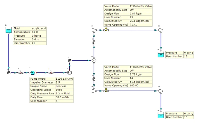
Figure 2.1: Acrylic Valve Turndown Model.
Before we write our script, let’s take note of some model-specific data (Table 2.1).
Table 2.1: Node Data
| Node Description | Node User Number | Design Flow rate (kg/s) |
|---|---|---|
| Centrifugal Pump | 4 | N/A |
| Butterfly Control Valve | 13 | 2.87 |
| Butterfly Control Valve | 14 | 5.75 |
The centrifugal pump has an operating speed range of 2850 to 1450 RPM. It is intended to run the simulation starting at the maximum speed of 2850 RPM and reduce the pump speed in steps of 20 RPM.
Let’s now consider writing the script in Pascal. Note, any text in blue below is supplementary and not included as part of the actual script.
Before we start, we need to set the programming language for the script. To do this, select: Script | Pascal (or Basic) from the Script window (Figure 2.2).
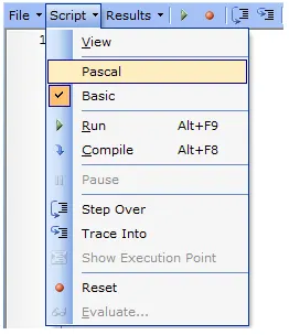
Figure 2.2: Pascal/Basic Script Setup.
- Acrylic Valve Turndown – Pascal.
|
Script |
Description of Script Steps |
begin |
Initialize the pump speed and other variables. Note, we need to give consideration to the descriptive terms we use here as they will form a key part of the script used later. (2850 RPM Max. Pump Speed).(1450 RPM Min. Pump Speed). (20 RPM Speed Decrement reducing from Max to Min Speed). Note, the pump in this model is a Peerless 8196 1.5x3x6 model and the capacity curve for this pump model is defined in the pumps database. |
Output.Clear; |
Clear the output window and chart results. |
Network.Set(4, 'BoosterOperatingSpeed', PumpSpeed);
|
Reset the pump speed and recalculate in case we have made previous calculation runs. The number 4 in this line refers to the User Number of the pump (unique node number – available from Results tab). Now, we need to set the pump operating speed (initial starting speed). We can retrieve the relevant property from the Helpfile. This data can be found at: Contents | Script References | Property Constants | Boosters. We can see from the list that what we need is Property Id 173 “BoosterOperatingSpeed“. The initial booster operating speed can be set to 2850 RPM by adding the term “PumpSpeed” to the script (“PumpSpeed” is 2850 RPM as described at the start of the script). |
Network.Calculate; |
Calculate the network. |
while ((PumpSpeed > MinOpSpeed) and |
Make the main loop using a while statement. Note the “and” condition in the “while” statement. The numbers 13 and 14 refer to the User Number of the control valves. The scenario we are creating here is, as long as the pump is operating at a speed greater than the minimum speed and the position of both control valves is below 100% fully open, run the simulation loop. Note, much like the pump, we have retrieved the relevant valve opening property from the Helpfile. This data can be found at: Contents | Script References | Property Constants | Controllers.
We can see from the list that what we need is Property Id 167 “CalculatedValveOpening“. |
begin |
Calculate the network. |
Results.Update; |
Update the chart results by including. |
PumpSpeed := PumpSpeed - SpeedDecrement; |
Now we need to reduce the pump speed from the initial starting speed which has been set in the script (2850 RPM). We can therefore use the descriptive terms we have used at the beginning of this script. |
Network.Set(4, 'BoosterOperatingSpeed', PumpSpeed); |
We need to update the reducing pump speed in the network during the simulation. |
(PumpSpeed <= MinOpSpeed) then
|
Now we can consider the results for the simulation. Write the result summary to a message box. The condition we are considering here is; if the network runs through the simulation and both valves are in control for all pump speed conditions, a message box will appear advising: ‘The system is able to control at the minimum operating speed of the pump'. However, this may not actually be the case so we need to include the conditions where either of the valves reach100% fully open before the pump reaches its minimum speed. Let’s consider the next line of the script. |
else |
Now we are considering the condition where either of the valves reach 100% fully open (more specifically, over 99% open) prior to the pump reaching its minimum speed, i.e. either of the valves lose control of the set flow rate. |
Network.Refresh; |
Refresh the network and results |
- Acrylic Valve Turndown – Basic.
|
Script |
Description of Script Steps |
PumpSpeed = 2850
|
Initialise the pump speed and other variables. Note, we need to give consideration to the descriptive terms we use here as they will form a key part of the script used later. (2850 RPM Max. Pump Speed).(1450 RPM Min. Pump Speed). (20 RPM Speed Decrement reducing from Max to Min Speed). Note, the pump in this model is a Peerless 8196 1.5x3x6 model and the capacity curve for this pump model is defined in the pumps database. |
Output.Clear |
Clear the output window and chart results. |
Network.Set(4, “BoosterOperatingSpeed”, PumpSpeed)
|
Reset the pump speed and recalculate in case we have made previous calculation runs. The number 4 in this line refers to the User Number of the pump (unique node number – available from Results tab). Now, we need to set the pump operating speed (initial starting speed). We can retrieve the relevant property from the Helpfile. This data can be found at: Contents | Script References | Property Constants | Boosters.
We can see from the list that what we need is Property Id 173 “BoosterOperatingSpeed“.
The initial booster operating speed can be set to 2850 RPM by adding the term “PumpSpeed” to the script (“PumpSpeed” is 2850 RPM as described at the start of the script). |
Network.Calculate; |
Calculate the network. |
WHILE ((PumpSpeed > MinOpSpeed) AND
|
Make the main loop using a while statement. Note the “and” condition in the “while” statement. The numbers 13 and 14 refer to the User Number of the control valves. The scenario we are creating here is, as long as the pump is operating at a speed greater than the minimum speed and the position of both control valves is below 100% fully open, run the simulation loop. Note, much like the pump, we have retrieved the relevant valve opening property from the Helpfile. This data can be found at: Contents | Script References | Property Constants | Controllers.
We can see from the list that what we need is Property Id 167 “CalculatedValveOpening“. |
Network.Calculate |
Calculate the network. |
Results.Update |
Update the chart results by including. |
PumpSpeed = PumpSpeed - SpeedDecrement |
Now we need to reduce the pump speed from the initial starting speed which has been set in the script (2850 RPM). We can therefore use the descriptive terms we have used at the beginning of this script. |
Network.Set(4, “BoosterOperatingSpeed”, PumpSpeed) |
We need to update the reducing pump speed in the network during the simulation. |
PumpSpeed <= MinOpSpeed) THEN
|
Now we can consider the results for the simulation. Write the result summary to a message box. The condition we are considering here is; if the network runs through the simulation and both valves are in control for all pump speed conditions, a message box will appear advising: ‘The system is able to control at the minimum operating speed of the pump'. However, this may not actually be the case so we need to include the conditions where either of the valves reach100% fully open before the pump reaches its minimum speed. Let’s consider the next line of the script. |
ELSE |
Now we are considering the condition where either of the valves reach 100% fully open (more specifically, over 99% open) prior to the pump reaching its minimum speed, i.e. either of the valves lose control of the set flow rate. |
Network.Refresh |
Refresh the network and results |
- Acrylic Valve Turndown – Results.
Now we can start the script simulation by clicking the Run button as shown below.

Figure 2.3: Script Run Icon.
When you select Run, the model will run through a series of iterations for each decremented pump speed. Control valve 14 reaches the fully open position (100% open) when the pump reaches a speed of 1970 RPM.
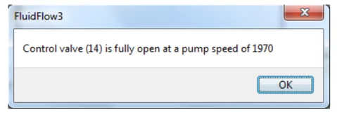
Figure 2.4: Script Message Box.
We can also view the pump and valve performance curves (based on a decrement of 20 RPM) by selecting: Results | View from the Script Window (see below).
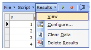
Figure 2.5: Results Data.
Firstly, you will see the graph plot of the pump performance which will be a linear plot since we are reducing the speed in constant steps of 20 RPM (see below).

Figure 2.6: Pump Performance Curve.
To view the performance curve for the valves, select the drop-down menu as shown below and choose the valve of interest.

Figure 2.7: Drop-Down Menu for Graph Plots.
Below is the performance curve for valve node 13 in this case which as we can see, reached approximately. 75% open when the simulation stopped (stopped as valve 14 was fully open at this point).

Figure 2.8: Valve 13 Performance Curve.
Finally, we have the performance curve for valve node 14 which reached the fully open position at 1970 RPM (see below).

Figure 2.9: Valve 14 Performance Curve.
You can edit the setup of your charts by selecting: Results | Configure (Figure 2.10).
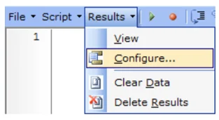
Figure 2.10: Configure Charts.
There are three charts for this particular example as shown in Figure 2.11.
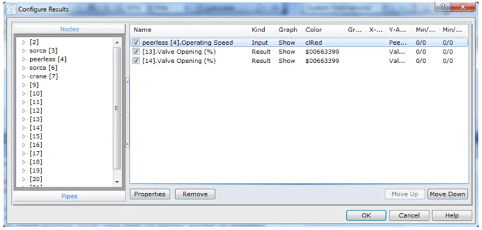
Figure 2.11: Configure Chart Display.
If you select any of the three charts, you can click the properties button which opens a new dialog as per Figure 2.12.
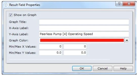
Figure 2.12: Result Field Properties Dialog.
You can edit the chart display and add labels to the chart from this dialog.
Note, this example file has been installed with your trial copy of FluidFlow. You can access the script for this example at:
- C:\Program Files (x86)\Flite\FluidFlow3\QA Scripting\Pascal\Acrylic Supply Control Valve Turndown
- C:\Program Files (x86)\Flite\FluidFlow3\QA Scripting\Basic\Acrylic Supply Control Valve Turndown (BASIC)
3. Butterfly Valve Pressure Loss vs Opening Position Script (Pascal)
This example shows how to plot a chart of pressure loss across a manual butterfly valve as a percentage of opening. We also wish to display the pressure loss results in kPa units. All results after a calculation are stored as SI values, this means that all pressure loss values are stored as Pa. If we just wish to display pressure loss in Pa we can use the Result Properties Dialog to automatically set up this column. Since we need to process the pressure loss results we must write a few lines of script to do this for us.
In this example there is no need to explicitly declare any variables but we will be using a reference to color variables and therefore we need to include Graphics in a uses clause.
The model of the system is shown in Figure 3.1.

Figure 3.1: Butterfly Valve Model.
Before we start, we need to set the programming language for the script. To do this, select: Script | Pascal (or Basic) from the Script window (Figure 3.2). In this case, we are selecting Pascal.
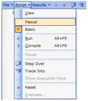
Figure 3.2: Pascal/Basic Script Setup.
- Butterfly Valve Pressure Loss vs Opening Position – Pascal.
| Script | Description of Script Steps |
|---|---|
uses Graphics; |
As we will be using a reference to color variables we need to include Graphics in a uses clause. |
begin ValveOpening := 100; MinimumValveOpening := 10; IncrementalChange := 2.5; PressureLossInkPa := 0; |
Initialise variables we will use. |
**Output.Clear Results.Clear** |
Clear and previous results. |
Network.Set(2,'ManualValveOpening', ValveOpening); Network.Calculate; |
Set the initial manual valve opening to fully open. |
PressureLossColumn := Results.Add('Pressure Loss (kPa)', True, clWebRoyalBlue, 'Valve Total Pressure Loss', 'Valve Opening 100 -> 5 in 2.5 increments', 'Pressure Loss in kPa'); |
Add a new field (PressureLoss) to be shown on the chart in blue. See the Results.Add method in the help file for information on the parameters together with additional sample code. |
while (ValveOpening >= 5) do begin Network.Calculate; NextRowIndex := Results.Update; |
Loop to change the valve opening. |
PressureLossInkPa := Units.Convert('Pa', 'kPa', Network.Get(2, 'PressureLoss')); Results.Set(PressureLossColumn, NextRowIndex, PressureLossInkPa); |
Set the pressure loss column values in kPa after conversion. |
ValveOpening := ValveOpening - IncrementalChange; Network.Set(2, 'ManualValveOpening', ValveOpening); end;end; |
Change the valve opening. |
- Butterfly Valve Pressure Loss vs Opening Position – BASIC.
| Script | Description of Script Steps |
|---|---|
uses Graphics |
As we will be using a reference to color variables we need to include Graphics in a uses clause. |
ValveOpening = 100 MinimumValveOpening = 10 IncrementalChange = 2.5 PressureLossInkPa = 0 |
Initialise variables we will use. |
**Output.Clear Results.Clear** |
Clear and previous results. |
Network.Set(2,”ManualValveOpening”, ValveOpening) Network.Calculate |
Set the initial manual valve opening to fully open. |
PressureLossColumn = Results.Add(“Pressure Loss (kPa)”, True, clWebRoyalBlue, “Valve Total Pressure Loss”, “Valve Opening 100 -> 5 in 2.5 increments”, “Pressure Loss in kPa”) |
Add a new field (PressureLoss) to be shown on the chart in blue. See the Results.Add method in the help file for information on the parameters together with additional sample code. |
WHILE (ValveOpening >= 5) Network.Calculate NextRowIndex = Results.Update |
Loop to change the valve opening. |
PressureLossInkPa = Units.Convert(”Pa”, “kPa”, Network.Get(2, “PressureLoss”) ) Results.Set(PressureLossColumn, NextRowIndex, PressureLossInkPa) |
Set the pressure loss column values in kPa after conversion. |
ValveOpening = ValveOpening - IncrementalChange Network.Set(2, “ManualValveOpening”, ValveOpening) END WHILE |
Change the valve opening. |
- Valve Pressure Drop – Results.
Now we can start the script simulation by clicking the Run button as shown below.

Figure 3.3: Script Run Icon.
When you select Run, the software will automatically run through a series of iterations. When complete, you can view the graph results by selecting: Results | View from the Script window.
You will firstly be presented with the graph result for the % opening position of the valve which is changing in steps of 2.5% as set in the script code. Since we have a constant % change, we have a linear type graph plot as shown in Figure 3.4.

Figure 3.4: Valve Position Chart Result.
If we select the drop-down menu (Figure 3.5), we can select the graph for valve pressure loss in kPa.

Figure 3.5: Chart Results.
Selecting Pressure Loss (kPa) reveals the chart result as shown in Figure 3.6.

Figure 3.6: Valve Pressure Loss Chart Result (kPa).
Note, this example file has been installed with your trial copy of FluidFlow. You can access the script for this example at:
- C:\Program Files (x86)\Flite\FluidFlow3\QA Scripting\Pascal\Pressure Loss v's Opening for a Manual Butterfly Valve
- C:\Program Files (x86)\Flite\FluidFlow3\QA Scripting\Basic\Pressure Loss v's Opening for a Manual Butterfly Valve
4. Orifice Pressure Drop Script with Excel Report (Pascal)
In this example, we have a digestion and flash tank plant with two-phase liquor entering the system with a set pressure of 2975 kPa g. We wish to write a script to predict the pressure loss across the orifice plate based on upstream pressure, flow and quality. Note, the quality shall change from 0.01 to 0.012.
The model of the system is shown in Figure 4.1.
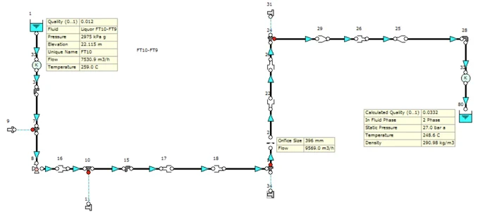
Figure 4.1: Digestion & Flash Tank System.
An Excel spreadsheet (titled ‘Orifice Pressure Drop’) is saved to the hard drive where we have stored the Input information for the model. The image below provides an overview of this data.
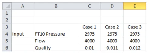
Figure 4.2: Excel Data to be used in simulation.
- Orifice Pressure Drop – Pascal.
| Script | Description of Script Steps |
const ExcelFileFolder = 'C:\A1\' ExcelFileName = 'Orifice Pressure Drop'; |
Define the constants to be used in the script. ExcelFileFolder denotes the filepath of the Excel file which contains data you wish to import to the simulation. Note, you will need to change this filepath to reflect the position where you are storing your .xlsx file. ExcelFileName denotes the name of the Excel file which you wish to use as part of the simulation. |
InputDataColumnStart = 3; InputDataRowStart = 3;PressureRow = 4; QualityRow = 6; |
Denotes the Excel start column (column C) of the input data. Denotes the Excel start row (row 3) of the input data. Denotes the row that holds the pressure data. Denotes the row that holds the quality data. |
SupplyNodeID = 1; OrificeID = 21; |
SupplynodeID: is the number FluidFlow assigns to the node where we wish to change values. OrificeID is the node number of the node whose results we are interested in. The orifice plate User Number is 21. |
OrificeTotalPressureLossRow = 10;OrificeFlowRow = 11;OrificeInQuality = 12; OrificeOutQuality = 13; |
Declare the rows where we want the results to start in Excel. Add more property rows here and then add a row for each addition in the WriteResultDescriptions and ProcessCaseStudies procedures. |
var objXL; |
Declare variables that will be used in the calculation. |
procedure StartExcel;var EmptyParam: OleVariant;begin objXL := CreateOLEObject('Excel.Application'); objXL.Visible := True; XLWorkBooks := objXL.WorkBooks; XLWorkBooks.Open(ExcelFileFolder+ExcelFileName, EmptyParam, EmptyParam, EmptyParam, EmptyParam, EmptyParam, EmptyParam, EmptyParam, EmptyParam, EmptyParam, EmptyParam);end; |
Start Excel Workbook. |
procedure StopExcel; begin objXL := UnAssigned;end; |
Stop Excel Workbook. |
function GetColumnCount: Integer;var col: Integer; |
This returns the number of columns in the result set. |
begin Result := 0; col := InputDataColumnStart; while (Length(obJXL.Cells[InputDataRowStart, col].Value) > 0) do begin Inc(col); Inc(Result); end;end; |
procedure WriteResultDescriptions;const ResultDescriptionColumn = 2;begin objXL.Cells[OrificeTotalPressureLossRow, ResultDescriptionColumn].Value := 'Orifice Loss (Pa)'; objXL.Cells[OrificeFlowRow, ResultDescriptionColumn].Value := 'Orifice Flow (kg/s)'; objXL.Cells[OrificeInQuality, ResultDescriptionColumn].Value := 'Orifice In Quality'; objXL.Cells[OrificeOutQuality, ResultDescriptionColumn].Value := 'Orifice Out Quality';end; |
The column title is assigned here. For instance, the Excel row for orifice total pressure loss will be described as ‘Orifice Loss (Pa)’. |
procedure ProcessCaseStudies;const InputTwoPhaseQuality = 69;var currentColumn: Integer; nDataColumns: Integer; thisPressure, thisQuality: Double; |
nDataColumns is the number of columns of data we have. This is the number of case studies. |
begin WriteResultDescriptions; nDataColumns := GetColumnCount; for currentColumn := InputDataColumnStart to InputDataColumnStart + nDataColumns - 1 do begin thisPressure := objXL.Cells[PressureRow, currentColumn].Value; thisQuality := objXL.Cells[QualityRow, currentColumn].Value; Network.Set(SupplyNodeID, 'BoundaryPressure', thisPressure); Network.Set(SupplyNodeID, InputTwoPhaseQuality, thisQuality); Network.Refresh; Network.Calculate(True); Results.Update;objXL.Cells[OrificeTotalPressureLossRow, currentColumn].Value := Network.Get(OrificeID, 'PressureLoss'); objXL.Cells[OrificeFlowRow, currentColumn].Value := Network.Get(OrificeID, 'InternalFlow'); objXL.Cells[OrificeInQuality, currentColumn].Value := Network.Get(OrificeID, 'TwoPhaseQuality'); objXL.Cells[OrificeOutQuality, currentColumn].Value := Network.Get(OrificeID, 'OutTwoPhaseQuality');end;end; |
GetColumnCount refers to getting the number of case studies we need to process. thisPressure refers to reading the pressure variable data from Excel. thisQuality refers to reading the quality variable data from Excel. Change the Input Data. Recalculate. Write Out the newly calculated results to Excel - All Results are returned in SI Units. (If we wish to display in any other units, refer to the example in the help file at: Scripting | Scripting Objects | Units Object). |
begin StartExcel; try ProcessCaseStudies; finally StopExcel; end;end. |
Script code execution starts here. |
- Orifice Pressure Drop – Results.
Now we can start the script simulation by clicking the Run button as shown below.

Figure 4.3: Script Run Icon.
When you select Run, the software will automatically start the relevant Excel file and use the data contained in this file to perform the simulation. The results will also be exported to the same Excel file based on the settings assigned in the script code.
The Excel report appears as shown below.
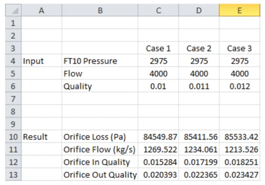
Figure 4.4: Excel Input and Results Data.
5. Mine Dewatering Script with Excel Report (Pascal)
In this example, we wish to consider the optimum pump speed and most cost-effective means of mine water removal using any number of pumps up to a maximum of 7 pumps (in parallel).
This system involves the transportation of mine water from an elevation of 4 M to an elevation of 30 M over a distance of approximately 364 M. As part of this script, we will export a unique set of results to an Excel report.
The model of the system is shown in Figure 5.1.
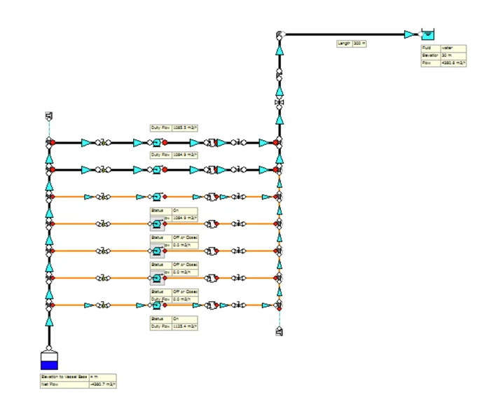
Figure 5.1: Mine Water Removal Plant.
- Mine Dewatering – Pascal.
|
Script |
Description of Script Steps |
const
|
Define the constants to be used in the script. Note, we need to give consideration to the descriptive terms we use here as they will form a key part of the script used later. (1480 RPM Max. Pump Speed which is fixed by the pump manufacturer).(900 RPM Min. Pump Speed. Below this figure the pump has insufficient head to overcome the discharge static height). (20 RPM Speed Increment increasing from Min to Max Speed). Note, all pumps in this network are Flygt CP3231 OOO*(450, 170kW) model and the capacity curve for this pump is defined in the database. |
xLColumnWidth = 12;
|
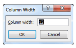
This is where we declare the setup of our Excel file which we will generate with the script. Note, the Excel report will be created automatically by the software. xLColumnWidth = 12; - This sets the width of the Excel column to 12 (see below).
xLColumnStart = 1; - This sets the results to start at column 1. |
var |
Declares the variables for the simulation. nPumps denotes the number of pumps under consideration. PumpCurrentSpeed denotes the current speed of the pumps. |
PumpId;
|
PumpId denotes a variant array of element numbers. PumpBESpeed denotes an array to hold the speed of the lowest specific energy (i.e. speed of BEP). |
procedure SetPumpSpeed(PumpNo, Speed: Integer); |
Helper Methods. |
procedure TurnPumpOn(PumpNo: Integer); |
The script will start by turning the pumps on and then to end the script simulation, turn the pumps off. |
procedure TurnPumpOff(PumpNo: Integer); |
The script will start by turning the pumps on and then to end the script simulation, turn the pumps off. |
procedure GetPumpValues(PumpNo: Integer; var Q, Eff, P, SpecificP: Double); |
Setup the calculation procedure. |
begin |
This represents the start of the main execution point where we initialise local variables. The row and column start point are obtained here based on the setup declared earlier in the script.
|
PumpId := [1,2,3,4,5,6,7]; |
Initialise all var arrays and pump status. PumpId denotes the unique pump user numbers (1 to 7). PumpBESpeed denotes an array to hold the speed of the lowest specific energy (i.e. speed of BEP). |
strPumps := ''; |
Determine how many pumps we wish to run. Note, a dialog box (Input Query) as shown below will appear asking how many pumps we wish to include in the simulation.
|
for i := 0 to nPumps - 1 do |
Update the array structures. |
objXL := CreateOleObject('Excel.Application');
|
Set up the Excel spreadsheet for results. |
objXL.Cells[xLRow, xLCol].Value := IntToStr(nPumps) + ' Pumps'; |
Write out the headers on the Excel sheet. |
try
|
Update results for current pump speed in the Excel report. |
XLCharts := XLSheet.ChartObjects; |
Set border of the chart. Produce the Excel chart. |
finally |
Tidy Up the Excel report.
|
- Mine Dewatering – Results.
Select Run from the Script window as shown below.

Figure 5.2: Script Run Icon.
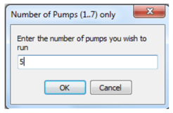
When you select Run, you will be presented with a dialog asking how many pumps you wish to consider in the simulation (1 to 7 pumps). For the purposes of this example, we have entered 5 pumps and selected OK.
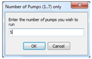
Figure 5.3: Number of Pumps to be considered.
The software will run through the simulation exporting results for Flow, Efficiency, Power and Specific Power to Excel. A graph curve relationship of specific power vs speed will also be generated from where you can clearly identify the most optimum specific power/speed. In this case with 5 pumps in operation, the optimum speed would be 1040 RPM as this produces the lowest specific power requirement (425 W/kg).
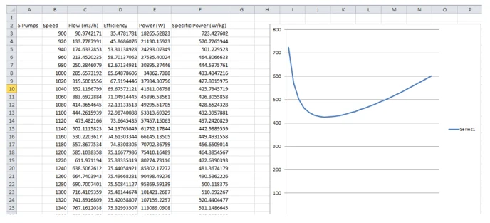
Figure 5.4: Excel Results - Specific Power vs Speed (5 Pump).
