Determining if a centrifugal pump curve suits your system can be a tedious process. The combination of different brands, models along with varying properties such as impeller size, speed, motor size and best efficiency point bring in countless options to choose from. 

This blog provides some hints and tips on how to check if a pump curve fits your intended system using FluidFlow. In case you need a refresher, a blog explaining centrifugal pump curves can be accessed here. 

The subsequent discussion takes reference on an Automotive Diesel Oil (ADO) Marine Loading system revamp project. This facility intends to load 500 m3/hr of ADO to 2 different piers located more than 1 kilometer apart using 2 parallel pumps. The modified loading network is designed to withstand 250 psig of pressure.

For this service, 3 x 250 m3/hr re-used centrifugal pumps will be installed with a performance curve shown in Figure 2. This pump allows up to 375 m3/hr of ADO throughput. 

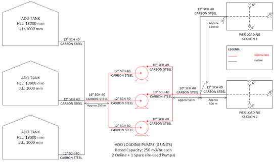
Figure 1: ADO Marine Loading System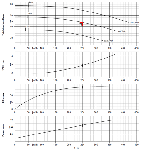

Figure 2: Candidate Pump Performance Curve

Using FluidFlow and available engineering documents such P&ID and piping isometric drawings, a detailed hydraulic model of the system presented in Figure 3 was developed to check the pump curve fit. Also entered in the hydraulic model are the details on the pump curve of flow versus head, NPSHr, and Efficiency as presented in Figure 4. 

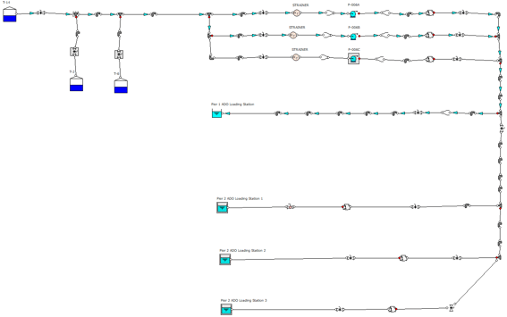
Figure 3: ADO Marine Loading System FluidFlow Model

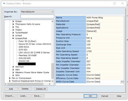
Figure 4: Marine loading pump curves in FluidFlow

Using  this example, we have created a list of our non-exhaustive tips on assessing pump curve fit using FluidFlow: 

1. Pump shut-off pressure 

In all of the tasks we do as Engineers, safety should be above all other requirements. For pumped systems, one way of practicing this is to ensure that the piping design pressure is always higher than pump shut-off pressure to prevent loss of containment.

The shut-off pressure is the resulting pump head when flow is zero due to a blocked discharge operation plus the maximum suction pressure. Each organization may have different means on determining the maximum suction pressure thus there is no standard way of calculating this parameter. 

In the example, let’s define maximum suction pressure as the sum of tank high liquid level difference from pump suction + Tank operating pressure. It’s relatively easy to determine this figure by hand calculation. However, if you want to use FluidFlow, all the user has to do is to input the high liquid level for the source tank and set the pump automatic sizing off with a pressure rise sizing model using the shutoff head differential as the setting. 

This will provide you with consistent units for the tank stagnation and pump differential pressures. Easily adding these values will give you the pump shutoff pressure. In the example, the results tab for the tank provided a stagnation pressure of 21.2 psig and a pump pressure rise of 57.5 psi. Combining these two figures, we get 78.7 psig which is lower than the system design pressure of 250 psig. Since the pump shutoff pressure is below system design pressure, the system is safe in case of a blocked pump discharge.

In some cases, careful consideration should be made especially for systems having alternative sections with different design pressures which can be the limiting condition.

The operating point of the pump at minimum conditions should be above the minimum allowable flow for the pump. Having this condition in reverse can lead to pump damage and potential system downtime. Further discussion on this topic flow can be found on our blog here.

In most cases, a pump minimum flow operation has already been defined for the vendor to consider. However, minimum flow operation from alternative or transient cases can be unseen and should be considered in the evaluation.

In the example, a transient minimum flow event has been defined. This occurs during initial loading where a maximum velocity of 1 m /s at the 6” discharge point is needed at a certain period. This is done to prevent fire hazard due to static charge accumulation caused by liquid velocity. During initial load, this translates to a flowrate of 65 m3/hr while the minimum allowable flow shown in the pump curve is 48 m3/hr as shown in Figure 2. Since the initial filling rate is higher than the allowable minimum flow, this would not be a limitation for the pump.

In some instances, an unintended possibility of operating below minimum flow can occur when the curve slopes are “too flat” which requires a deeper analysis. Further discussion on the pump curve slope is discussed on the succeeding sections.

3. System Curve

Except for a few cases on unit revamps, system curves in preliminary pump calculations are generated through a conceptualized pipe layout where lengths, equipment arrangement, elevations and fitting details are not yet final and most likely padded with large design margins. This is being done to cover for uncertainties or unexpected hardware changes in the project. Thus make a preliminary calculation of the pump differential head on the high side.

As the project progresses, pipe layout generated from plot plans become isometric drawings and vendor information for inline elements becomes available. This enables the development of a hydraulic model that could generate an accurate system curve and check if the proposed pump curve satisfies the following:

• Required pump output is met
• Duty point is reasonably near (usually +10%) the pump Best Efficiency Point (BEP)
• Control valves (if installed in the system) have enough pressure drop for satisfactory operation

Applying the items discussed in the example, pump performance was estimated to have a combined output of 648 m3/hr to the farthest Pier. This exceeds the required loading rate of 500 m3/hr as presented in Figure 5a.

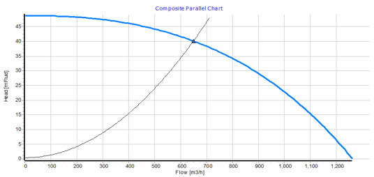
Figure 5a: Parallel Pump Composite vs. System Curve

Individual pump performance show that their individual duty points are at an efficient operating range of 79.7% vs. 81% (BEP) as presented in Figure 5b.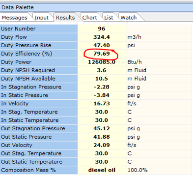 

Figure 5b: Individual Pump vs. System Curve

4. Pump Curve Slope

Typically, a 10 - 25% head rise from rated to zero flow generates a pump curve slope with adequate room for control. In some cases, pump vendors may offer models with a head rise to shutoff below 10% and results in a flatter curve slope.

A very “flat” curve slope for the pump means slight reduction in flow such as small valve turns or turning a parallel pump on could lead to operation below minimum allowable flow. 

The effect of flow disturbance on the slope of the pump curve can be assessed in a hydraulic model.  In the example, this can be done by simulating pump lower flow operating conditions such as:

• Running all pumps in parallel (due to pump switching) to the most restrictive normal path
• Pinching valve opening (5% open) while discharging to the most restrictive normal path
• Any other operating scenario leading to very low pump output deemed credible  

In the example, the first two conditions above were run in FluidFlow and yielded the following duty point shown in Figure 6 and 7.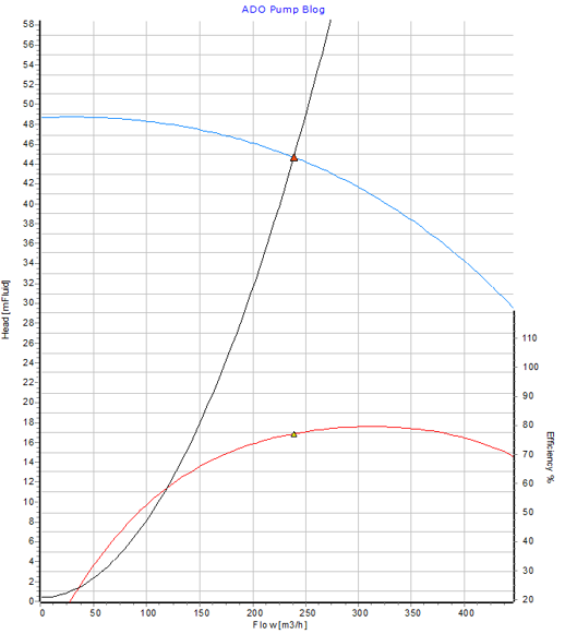

Figure 6:  Parallel operation of 3 pumps

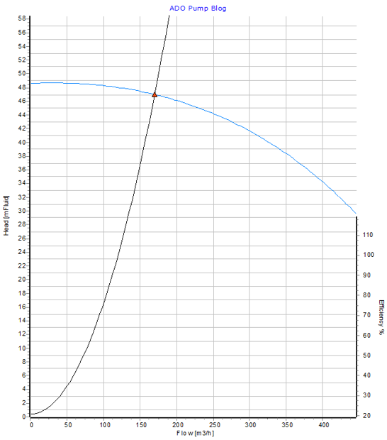Figure 7: Pinching one valve to 5% while 2 pumps discharge to 1 point

Under the harsh duty points simulated, the pump is expected to operate above the allowable minimum flow of 48 m3/hr. 

5. Pump End of Curve Performance

In most cases, the end of curve performance is checked to ensure the pump will not operate beyond what is recommended by the Vendor to ensure its reliability. This is most of the time performed on systems where the operating duty of the pump is uncontrolled either as intended or unforeseen. 

End of curve pump operation occurs when the system resistance is very low, it forces the pump to operate at its maximum output. Having this output might mean the pump is operating beyond its curve or its mechanical limits. One instance would be the sudden trip of parallel pumps, an alternative operating case with less flow restrictions or a “fail open” operation of a control valve. 

In our example, the head for 2 pumps operating in parallel at the required capacity of 250 m3/hr has been defined for the system. However, there are 2 destinations for this pump which are located far from each other. Since there is no flow control, pump operation floats on an uncontrolled system curve. When diverted to a closer or less restrictive path, pump will be forced to operate to the right side of the curve. Hence, pump end of curve performance needs to be checked.

Figure 8 shows the pump operating above 400 m3/hr. This exceeds the maximum allowable flow of 375 m3/hr when configured to deliver to Pier 2: 

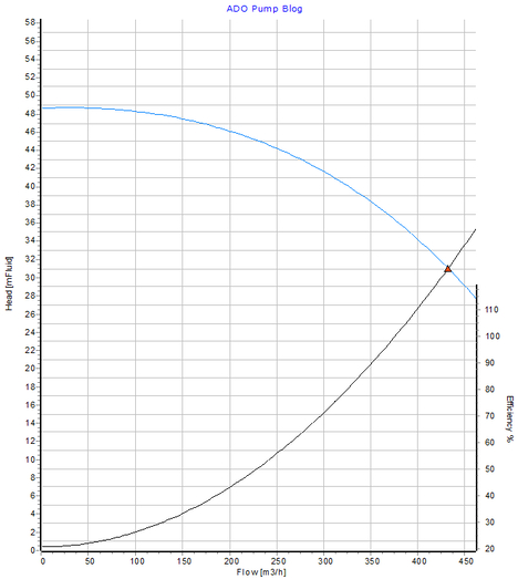 Figure 8: Dual and Single Pump Performance vs. System Curve

6. Pump NPSHr vs NPSHa

The Net positive suction head required (NPSHR) varies with the duty point of the pump. If this is higher than the Net positive suction head available (NPSHa), cavitation would occur which can damage the pump. This should be checked along with the head curve especially when the pump could be operating above its rated output.

In our example, it has been established that the pump can operate beyond its required throughput. With the NPSHR curve entered in the database, FluidFlow automatically makes this comparison and prompts a warning message if NPSHA is lower than NPSHR as shown in Figure 9.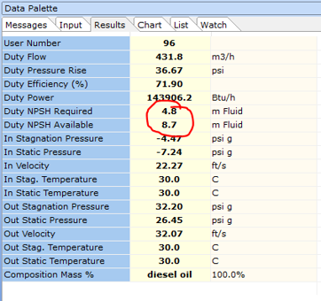

Figure 9: NPSHR vs. NPSHA Comparison in FluidFlow

Conclusion

In general, the “fit” of a pump curve depends greatly on the requirements of your system which should be defined as accurately as possible. It is important that the operating intent for the pump is clearly understood before sizing and alternative scenarios are defined for consideration. The following as a minimum should be checked with the pump curve:

• Pump meets its required output
• Pump shutoff pressure is equal or lower than the system design pressure
• Pump will be operating not lower than the allowable minimum flow
• Normal pump operation is close to Best Efficiency Point (BEP) as possible
• There is enough head rise between zero to rated flow to cater for unexpected reductions in flow that can cause it to operate below minimum flow
• There is enough pressure drop for control valves to operate effectively
• NPSHa is higher than NPSHr in all operating cases

There are instances where a pump end of curve performance is checked to ensure it will not operate beyond what is recommended by the Vendor. This happens on systems where the pump output is uncontrolled either by design or unintended. Simulating an end of curve pump operation should be performed to determine if an “out of curve” condition is possible.

A powerful hydraulic tool such as FluidFlow is important to ensure a reliable conclusion is formulated through an accurate hydraulic model.